Profluent has announced their new family of foundation models for protein generation, the ProGen3 series.

Whether you’re looking to understand their methods and findings, or simply curious on what the heck a protein language model is –– you’re in the right spot.

If you haven’t seen it yet, I encourage you to watch this short clip/teaser released by the Profluent team:

We’ll start simple.

So…

What even is a protein language model?

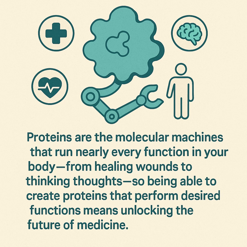
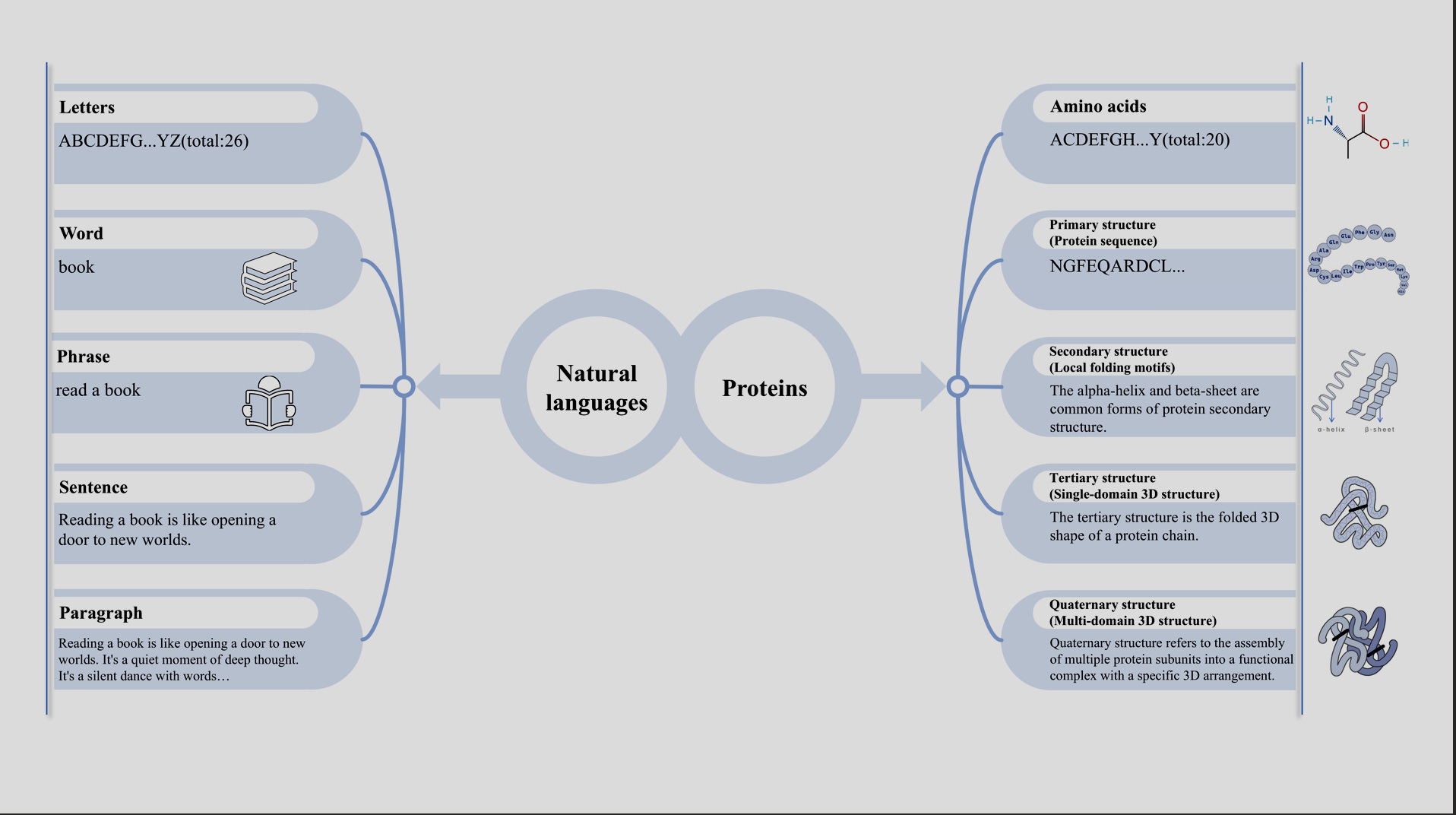
Imagine if proteins had their own version of English—except instead of letters, it's amino acids. And instead of grammar rules, it's evolutionary constraints and folding patterns.

A protein language model (PLM) is a neural network trained to understand the language of proteins. It looks at massive databases of protein sequences—in this case billions of sequences—and learns the patterns, structures, and "syntax" behind them.

Just like how GPT can write your The Catcher in the Rye essay, these models can generate brand-new proteins, fill in missing parts, or even predict how a change in sequence might affect function.

It’s like ChatGPT for biology—except instead of finishing your sentence, it might generate a life-saving enzyme.

And the twist: Creating a protein that will actually do what it’s supposed to do in your body–and not have any negative effects–is a lot more complicated than writing essays, or generating a character with 6 fingers like the one at the beginning of this article (did you notice?).

Subscribe now

The point is, with your typical large language models, we have a lot of room for error/mediocrity. With science, particularly medicine, we do not.

Thank you to the team at Profluent for their role in pushing the boundaries of science, and to everyone on X & Bluesky who I’ve had rich discussions with on this topic.

How we got here.

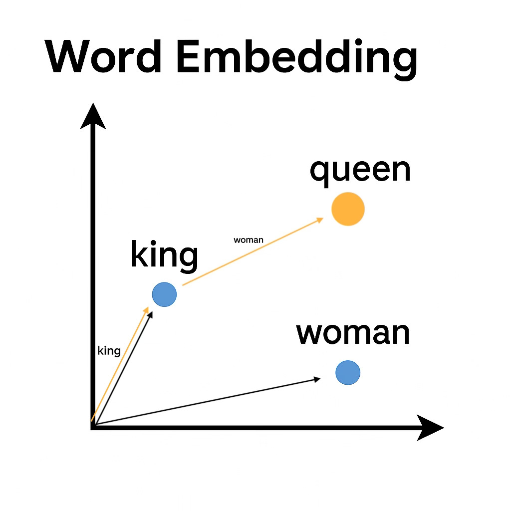
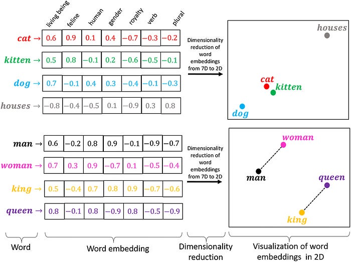
In the 2010’s, the idea that protein sequences could be modeled like language sparked a new wave of research. ProtVec was of the first to do it, building off of Google word2vec’s skip-gram model for mapping words to embeddings, and applying it to protein sequences in the Swiss-Prot dataset. Though ProtVec wasn’t a neural network language model in the modern sense, it was of the first to apply word embedding techniques to protein sequences, treating amino acid triplets (e.g. “CAU”) as "words" and generating distributed representations for them.

Another example:

In 2019, one of the earliest protein language models was a bi-directional long short-term memory (LSTM) embedding model:

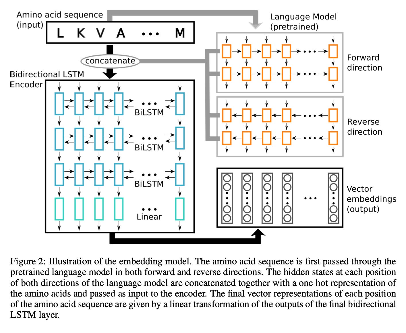
The result?

We started realizing neural networks could capture meaningful structural features of a protein from sequence data alone.

The early models laid the groundwork for what we have today.

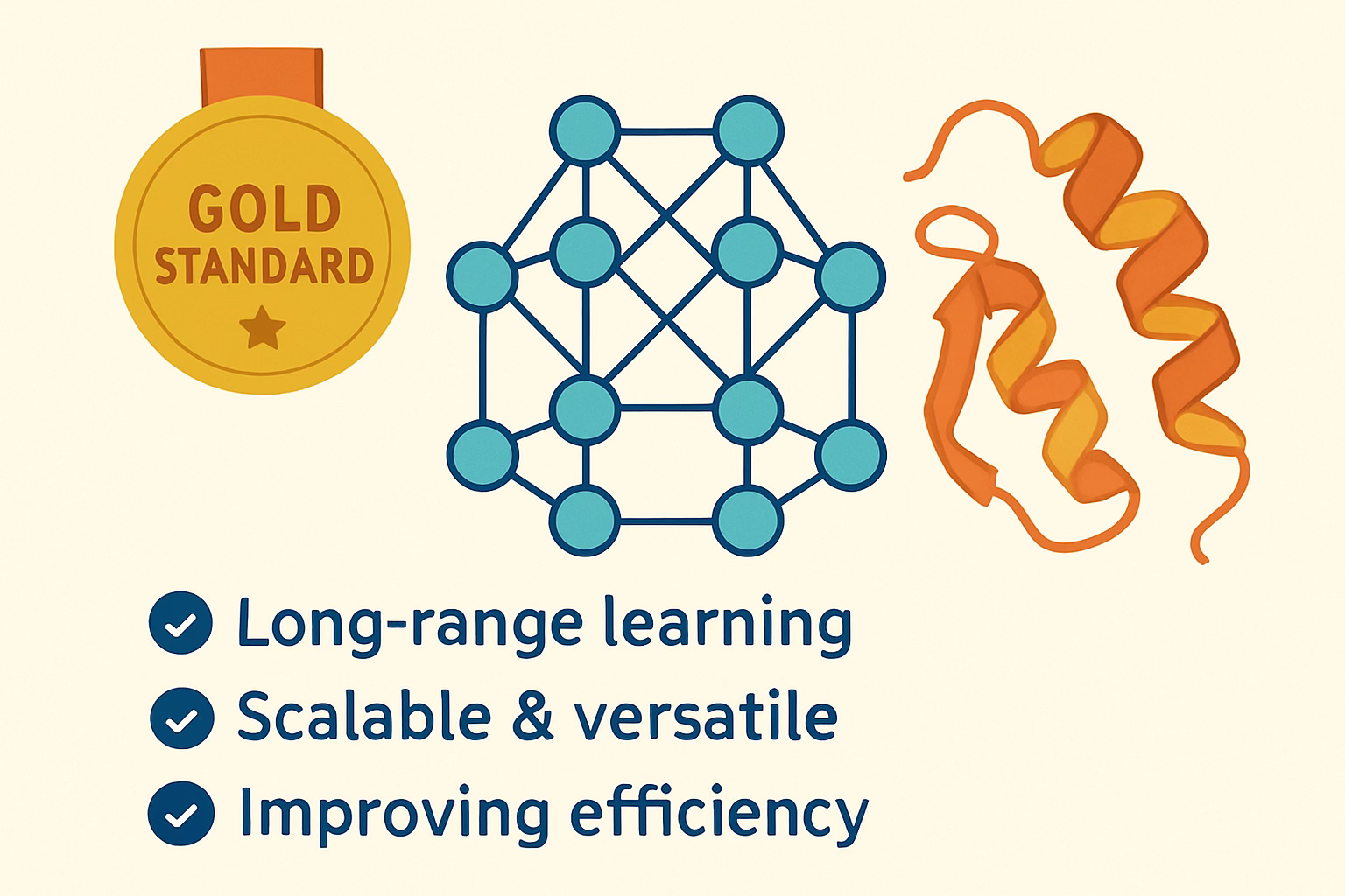
Transformer models, which you may know as the gold standard for LLMs, are also the gold standard for PLMs, for many reasons:

• They’re great at capturing complex, long-range relationships in protein sequences thanks to their self-attention mechanism, which enables them to learn evolutionary and co-variation patterns traditionally captured by multiple sequence alignments (MSAs, a computationally and time intensive step that requires searching through protein databases). In some cases, transformer models have even matched or outperformed MSA-based methods; Chai-1 is a good example of this, which I covered in my post about Foundation Models and Drug Discovery at NVIDIA GTC 2025.

• Their scalability and versatility allow training on massive protein datasets and adaptation to many bioinformatics tasks.

• Even though they are computationally expensive, ongoing research is making transformers more efficient and even more powerful for protein generation.

How do we make these things better?

Though there have been many studies on protein language models and sequence generation, some key questions stick out:

1. Optimal Training Data Distributions: How do different data sampling strategies affect model performance? Is there an optimal data distribution strategy here?

2. Scaling Laws: Is there a mathematical or empirical rule (a "scaling law") that predicts how performance improves as you increase model size or data? Do these laws mirror those seen in Natural Language Processing (NLP)?

3. Model Size and Performance:

   1. Foundational Capacity: Does increasing model size actually result in the generation of more diverse, novel, and experimentally viable proteins?

   2. Aligned Performance: How much better can bigger models get after fine-tuning/alignment with laboratory data?

Recent work — namely ProGen3 — takes direct aim at these questions. Profluent’s latest release explores how training data composition, model scaling, and laboratory validation play a role in pushing the frontier of protein generation. Here’s how they did it.

Making these things better.

Architecture breakdown

• Sparse Mixture‑of‑Experts (MoE) Transformer
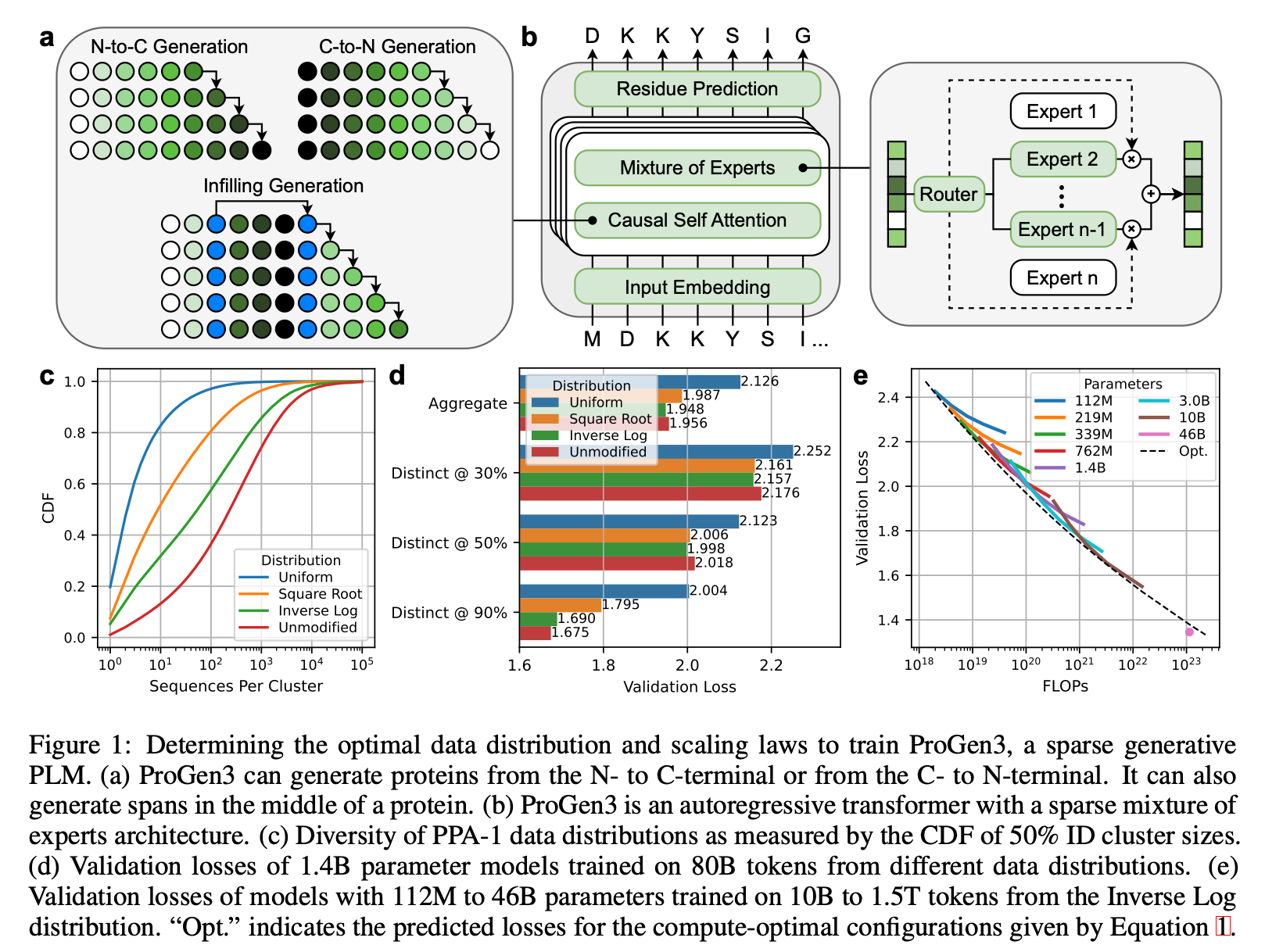
  ProGen3 uses an autoregressive (AR) Transformer with a sparse MoE setup. It activates only about 27% of parameters per forward pass. This cuts compute while letting the model scale effectively.

• Eight Model Sizes
  Parameter counts range from 112M → 46B, all sharing a 8,192‑token context window so long protein sequences fit natively.

• Why Sparse?
  For a fixed compute budget, sparse models outperform dense ones, mirroring trends in NLP.

• Two Generation Modes

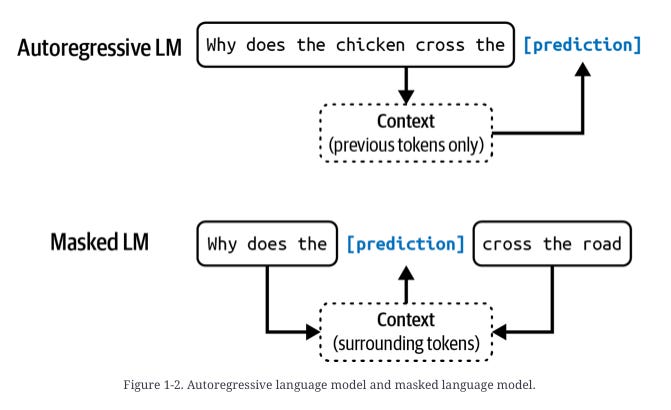
  1. Causal Language Modeling (CLM) – generates proteins residue‑by‑residue from either N→C or C→N direction. This is similar to autoregressive language models.

  2. Generalized Language Modeling (GLM) – in‑fill anywhere in the sequence: target spans are replaced with sentinel tokens, and the model predicts those spans in a trailing block, allowing domain‑level redesign while attending to full context. This is similar to masked language models.

Training Distribution

Q: Is there an optimal data distribution strategy?

Protein datasets have biases that influence the quality of PLMs trained on them. They seek to find optimal training data distributions to overcome these biases and boost the quality of PLMs.

To train ProGen3, they curated a new dataset— the Profluent Protein Atlas v1 (PPA-1). Quick breakdown of PPA-1:

• 3.4B proteins

• 1.1T amino acid tokens

• Includes wide range of genomic and metagenomic sources

• Considerably larger than UniRef and BFD.

• Multiple layers of quality filters:

  • excluded all protein fragments - they only wanted to train on full protein sequences. PPA-1 is of similar size as ESM3’s dataset, but ESM3’s includes protein fragments.

Proteins cluster into groups based on how similar their sequences are (e.g. 50% identity (ID) clusters). The authors explored four different strategies for picking training examples from these clusters, ranked from most diverse to least diverse:

1. Uniform: Sample every cluster equally, no matter how big or small. (most diversity, sampling from each group).

2. Square Root: Sample more from bigger clusters, but not proportionally — the bigger the cluster, the more, but gently (by √n).

3. Inverse Log: Sample almost proportionally to size, but slightly down-weight very large clusters.

4. Unmodified: Just sample naturally — big clusters dominate.

After training models of the same size on each distribution and comparing results for each model across the different distributions, they found:

• When generating proteins similar to those in your dataset (90% ID), the Unmodified strategy works best — because it mirrors natural frequencies.

• If you’re looking for very different, out-of-distribution proteins (30%-50% identity), Inverse Log works best — balancing between too much replication (over-representing very common protein families) and too much flattening (opposite of replication).

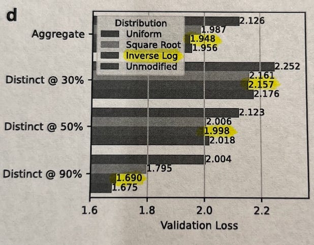
Uniform sampling — which might seem “fair” at first — actually performed the worst. This suggests that protein models need to "feel" the natural frequency of similar proteins to learn important biological patterns, but slight rebalancing helps them generalize better.

Because of this, they trained subsequent models using the Inverse Log sampling strategy — hitting the best balance between memorization and generalization. This choice is important because it prioritizes being able to use the model for proteins that are not well-represented in the training data, making these models more generalizable.

So, to answer the training data distribution question:

It depends on the task:

• Sample from the Unmodified distribution for incremental, low‑risk designs.

• Sample from the Inverse‑Log distribution when you need diversity and are willing to go further off the map.

Scaling up to 46B parameters

Q: Is there a mathematical or empirical rule (a "scaling law") that predicts how performance improves as you increase model size or data? Do these laws mirror those seen in NLP?

As your dataset grows, you would expect to need a bigger model, but how big is optimal?

To build better protein models efficiently, ProGen3 explores a key idea also present in NLP: scaling laws. These are formulas that help you figure out the best way to spend your compute budget — whether you should invest in a bigger model or more training data.

Here’s what they did:

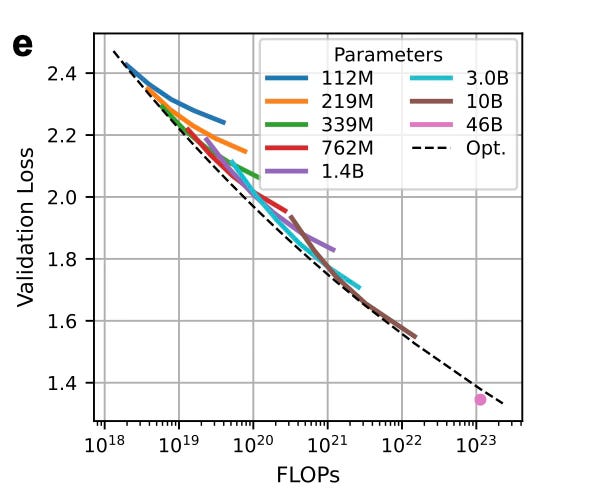
• They initially trained models ranging from 112M to 10B parameters, using datasets from 10B to 1T amino acid tokens.

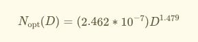
• Using results from each training run, they fit a scaling law equation (originally proposed by Kaplan et al) to predict validation loss as a function of model size (N) and dataset size (D).

• The resulting equation tells you the compute-optimal model size for any given dataset size:

  

  Proportionally speaking:

  

  For example, if you had 1.1×10²³ Floating Point Operations per second (FLOPs), the optimal setup would be a 90B parameter model trained on 753B tokens.

But they made a trade-off:

• Instead of pushing for the 90B model (which would be hard to run), they trained a 46B parameter model on 1.5T tokens, which fits on 4×A100 GPUs.

  

• This model still beat expectations — achieving a lower loss than predicted. They say it’s possibly due to training improvements like a longer warmup period.

They then shifted focus to in-vitro expression.

Larger PLMs generate more diverse proteins that express in vitro.

They focused on three models, separated by three orders of magnitude in pre-training compute, to evaluate diversity of proteins generated and their expression levels in vitro:

• ProGen3-339M (trained on 200B tokens with 1.2x10^²⁰ FLOPs)

• ProGen3-3B (trained on 500B tokens with 2.6x10^²¹ FLOPs)

• ProGen3-46B (trained on 1.5T tokens with 1.1x10^²³ FLOPs)

All three were pre-trained on PPA-1, applying the Inverse-Log strategy, to emphasize out-of-distribution coverage.

A quick recap of their methods / results:

Quality-filter pipeline

They applied a series of quality filters to extract “protein-like” sequences.

1. Language models often generate repetitive sequences, so they started by removing sequences in which >25% of the sequence consisted of low-complexity regions. 95.5% of the sequences in PPA-1 already pass this filter.

2. Generations must include the appropriate termination token.

3. Require >80% alignment coverage to any natural sequence from PPA-1.

What did they find?

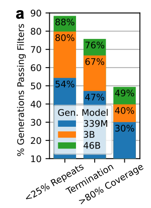
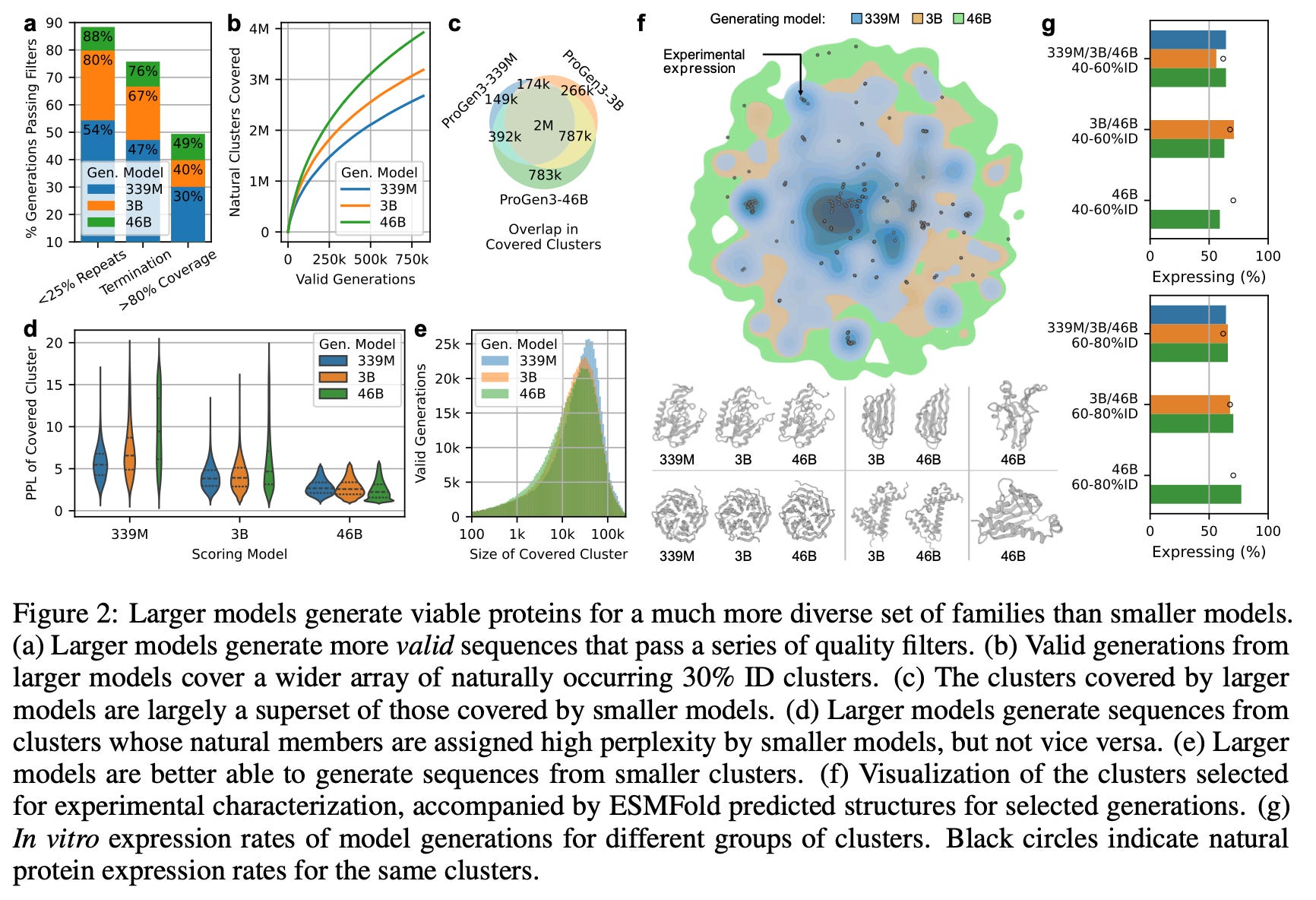
Larger models (46B) generate more valid sequences that pass each of these quality filters. Scaling up from 339M to 3B especially reduces the number of repetitive generations.

30% ID clustering analysis

Counting how many clusters get covered tells us how well the model explores known sequence space.

• They aligned every valid generation to the 30% ID cluster representatives of PPA-1.

• They labeled a sequence generation as ‘covering a cluster’ if it is ≥30% ID to the cluster representative with ≥90% alignment coverage.

What did they find?

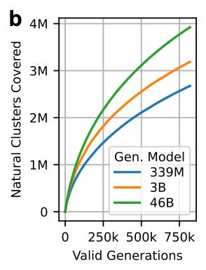
Larger models generate sequences from a more diverse set of clusters than smaller models.

Soluble Expression - Lab assay design

They chose the split-GFP E. coli expression assay to measure soluble protein abundance. Soluble protein abundance depends on factors like mRNA abundance and stability, translational yield, thermodynamic folding equilibrium, kinetic stability, toxicity, etc.

• This assay correlates well with protein expression assayed by direct methods like SDS-PAGE and Western blotting.

• It has also been used to benchmark generative protein models in previous works.

149 clusters were sampled in three tiers:

• 42 clusters in which all 3 models generated from

• 62 clusters that only ProGen3-3B and ProGen3-46B generated from

• 45 clusters unique to 46B.

From each cluster, they took two generated sequences per model:

• one moderately distant (40–60% ID) and

• one closer (60–80% ID)

They chose the candidate with the lowest perplexity, plus two random natural proteins as controls.

…What did they find?

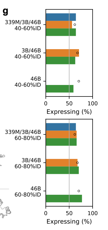
As expected, the 60–80% ID designs expressed better than the 40–60% set, but, more importantly, the synthetic proteins expressed about as well as the natural controls (black circles) from their own clusters.

In these split-GFP assays, all three models achieved similar overall expression rates, but the 46B model achieved that success across many more clusters.

But wait, wasn’t 46B evaluated across many more clusters than the other model sizes?

Yes, but 46B covered the same clusters the smaller models covered, and then some, and was still able to maintain impressive expression levels across each cluster.

In other words, 46B’s set of covered clusters is almost a superset of 3B, which is almost a superset of 339M. Smaller models never reach many of the clusters ProGen3-46B visits. See figures c, d, and e below 👇

So, with this, they showed the generated sequences make enough soluble protein to be purified and studied.

For an early screen of millions of de-novo sequences, that’s a pragmatic first hurdle.

Key distinction: expression ≠ viability, but confirming soluble expression is an essential precursor to any functional test. We’ll get to viability soon.

Beyond the comfort zone: <30% ID and infilling

After showing that from ≥40%–ID clusters as natural reference points the 46B model reliably generates proteins that fold and remain soluble, the authors asked a tougher question:

Can the models still produce soluble proteins when there is no natural reference point to lean on?

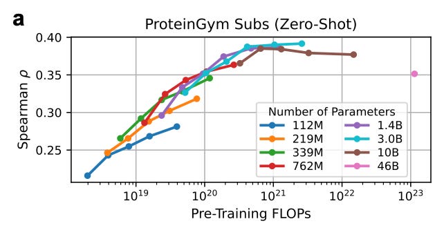
Specifically, they considered the set of sequences that had less than 30% ID to any protein in PPA-1, or that could not be aligned.

For each of the 3 models, they picked 30 generations (balanced across α, β and α/β folds, so 10 each here) for a total of 90 generations.

Then, they ran the same split-GFP assay.

What did they find?

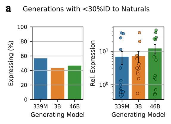
Looking at the chart on the left, the smallest model seems to have a better hit rate: it generates more sequences that express. On the right, we see the 46B model delivered a higher yield: of the designs that did express, expression levels were higher for 46B. But there isn’t a consistent trend.

They also took a few therapeutically and industrially relevant proteins, and assessed expression after long and short infilling tasks. They saw similar results:

This suggests that bigger models may also understand long-range context a bit better, which matters when you drop a novel motif into an existing fold.

Ok. That was a lot. What have we learned about scaling so far?

We revisit the main question that inspired this section:

Scaling ProGen3 from 339M to 3B and then to 46B parameters delivered three clear benefits, plus one important caveat.

First, sequence quality improves: the larger models produce far fewer low-complexity, repetitive, or poorly aligned chains, indicating that basic “protein grammar” is captured better as capacity grows. More sequences passed the filters.

Second, diversity explodes: when generations are mapped to 30%-ID clusters, the 46B parameter model covers almost every cluster reached by the smaller models and ventures into many new ones that the small models cannot access, a gap that sampling alone cannot close because the smaller models assign prohibitively high perplexity to those regions. Conversely, the smaller models never venture into the pockets of sequence space that the 46B model regards as highly improbable / high perplexity (figure 2d).

Third, breadth of in-vitro expression expands: split-GFP assays show similar overall expression rates across model sizes, but the largest model achieves those rates across a much wider range of sequences (figure 2). Even with <30%-ID to any protein in PPA-1, and across long- or short-span “in-filled” redesigns of existing proteins, the 46B parameter model generates proteins with higher relative expression.

Scaling buys a broader and deeper prior: the 46B parameter model can venture into low-identity territory and still yield proteins that fold and express, and it handles mid-sequence edits with slightly higher success.

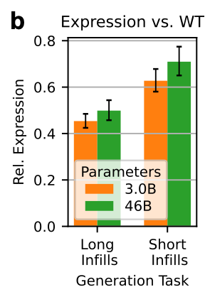
The caveat: The authors found models larger than 3B parameters actually slide backward in zero‑shot accuracy. Split‑GFP is a reliable first check for solubility and proper folding. But it says nothing about catalytic turnover or binding affinity, the functional qualities we ultimately need.

That is, beyond a certain threshold, better estimators of the natural protein distribution can be worse fitness predictors.

But that’s not the end of the story. 🥁🥁🥁

Alignment

Once the ProGen3 models are aligned to even modest amounts of laboratory data, the extra parameters that looked useless for zero‑shot fitness suddenly come alive.

Using Iterative Reasoning Preference Optimization (IRPO)—a lightweight fine‑tuning loop that nudges the model toward experimentally measured traits—the authors fed each model as few as 500 experimental measurements of single-substitution protein variants, and saw benefits in fitness prediction.

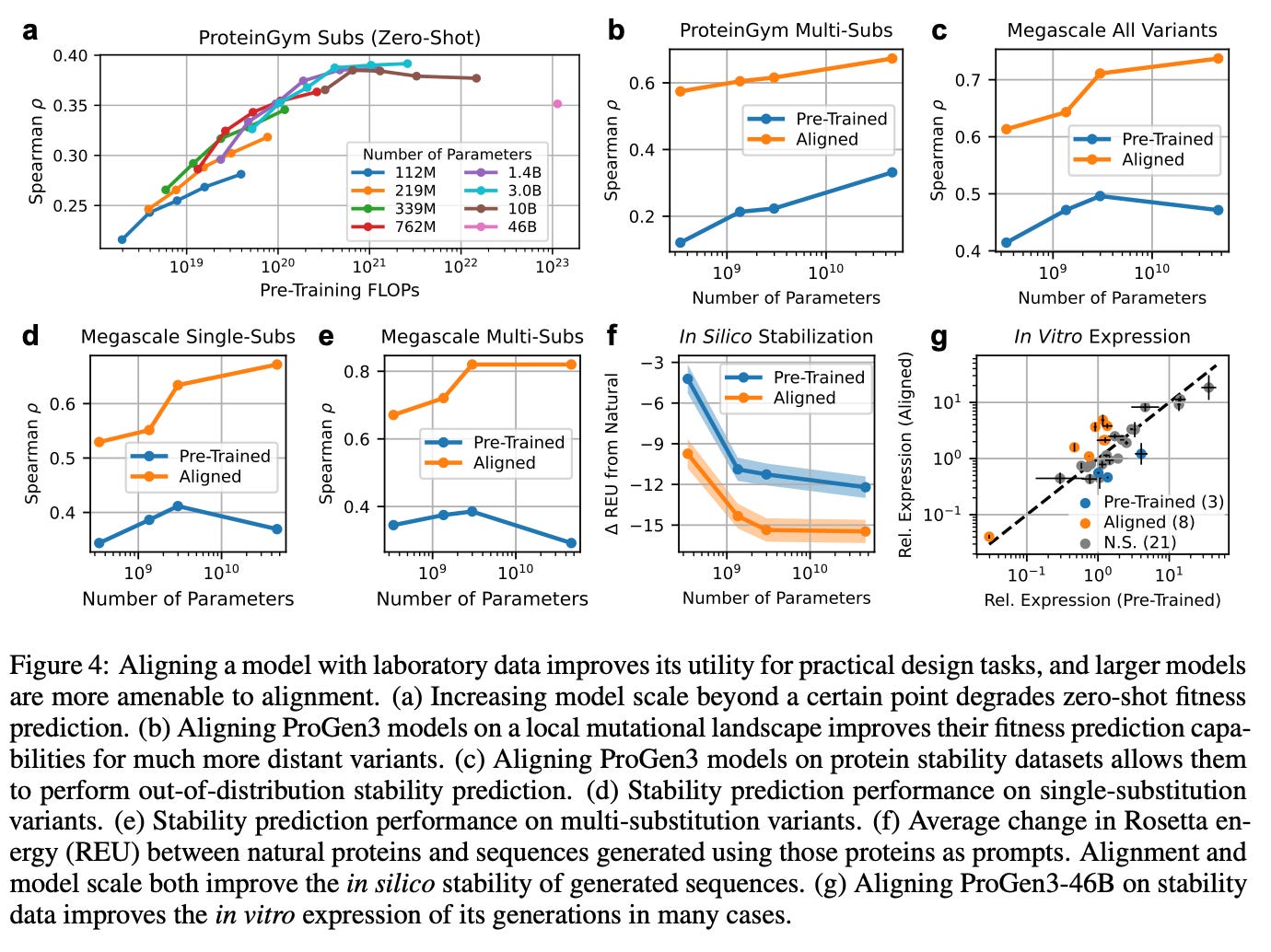
They rank the model’s predicted sequences by their likelihood, rank the same sequences by the fitness values measured in a deep‑mutational‑scan dataset, and then see how similar those two rankings are using the Spearman correlation (ρ).

That supervised nudge was enough for the 46B-parameter model (ρ = 0.673) to surpass and match state-of-the-art baselines like KERMUT (ρ = 0.628) and ConFit (ρ = 0.679), respectively, all while remaining a full sequence generator rather than a static scorer.

The same trick, applied to nearly 800,000 folding‑free‑energy (ΔG) measurements, taught the model a sequence‑only notion of stability that generalized to proteins it had never seen and held it up when the variants contained many simultaneous mutations.

On multi‑substitution variant stability, the aligned ProGen3‑46B reached a Spearman ρ of 0.82, leaving specialized structure‑aware baselines trailing far behind.

Alignment didn’t just sharpen the model’s predictions; it materially improved what the model makes.

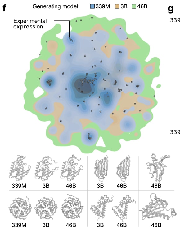
When the stability‑tuned 46B model generated 50,000 new sequences per prompt, from 32 structurally diverse natural proteins, the in-silico Rosetta energies shifted decisively toward lower (more favorable) values (figure 4f).

Split‑GFP screens back up the computation: in roughly 25% of the scaffolds the aligned 46B designs showed higher soluble yield than their pre‑trained counterparts—often matching or topping the wild type—while only three scaffolds saw a drop. So scale gives you the reach, but alignment gives you the steering wheel, turning raw statistical muscle into proteins that not only fold and express but start to edge toward real function.

The key insight from ProGen3: scale builds better priors — but you still need light supervision (e.g. IRPO) to unlock their full potential in biological settings.

In summary:

Is Bigger = Better in Protein Models?

Yes — for sequence modeling:

• Bigger models (like ProGen3’s 46B) consistently get lower perplexity, meaning they’re better at capturing the patterns of natural protein sequences.

• They also generate sequences with better diversity, stability, and expression — especially when aligned with a small amount of lab data.

No — not always for zero-shot biological tasks:

• On benchmarks like ProteinGym, bigger models don’t improve (and sometimes worsen) fitness prediction when used without fine-tuning.

• This is because they’re too good at modeling evolution — which doesn’t always match what a single lab assay is measuring.

Yes again — if lightly tuned:

• When a big model is aligned with just ~500 fitness labels (e.g. through IRPO), it can outperform smaller models and even specialized predictors.

• Scale gives a powerful foundation — but you still need to nudge it in the right direction.

Bigger models are better at learning biology — but not automatically better at doing what you want.
With the right nudge (in this case, small supervised alignment), scale can become a superpower.

This is just the beginning! If you enjoyed this read, please consider subscribing for more on AI and Drug Discovery.

Subscribe now